6. Benchmarks

In order to test the accuracy of the Mandyoc code, its results can be compared to benchmark studies. The following subsections will present the procedures and results for some well established modeling problems. Such cases should provide information about the applicability and performance of the code as well as some of its limitations.

The scripts to build and run these numerical experiments are located in the examples folder of the Mandyoc repository. Inside each example folder, you find a Jupyter notebook with detailed explanation and instructions on how to run the experiment.

6.1. van Keken et al. (1997) [20]

Note

Mandyoc version used for this benchmark: v0.1.4.

The set of simulations proposed by van Keken et al. (1997) [20] compares several methods of studying two dimensional thermochemical convection, where the Boussinesq approximation and infinite Prandtl number are used.

For this benchmark, the first case is presented with the three distinct variations, as proposed by the article. The simulation consists of two layers, where a buoyant thin layer is under a denser thicker package. The problem can be interpreted as a salt layer under a sediment package, and the interface between the layers is defined by the Eq. 6.1 below.

(6.1)\[y=-0.8 \lambda_y + 0.02 \cos{\frac{\pi x }{\lambda_x}}\]

where \(\lambda_x\) and \(\lambda_y\) are the horizontal and vertical lengths of the simulated 2-D box, respectively.

The simulations are carried out in a Cartesian box where the fluid is isothermal and Rayleigh-Taylor instability is expected for the proposed setup. The table below lists the parameters used to run this scenario together with the distinction between the three proposed simulation (case 1a, 1b and 1c).

Table 6.1 Parameters used for the Rayleigh-Taylor instability simulation.

Parameter	Symbol	Value
Horizontal length	\(\lambda_x\)	1.0000
Vertical length	\(\lambda_y\)	0.9142
Thermal diffusion coefficient	\(\kappa\)	\(1.0\times 10^{-6}\)
Gravity acceleration	\(g\)	\(10\)
Reference viscosity	\(\eta_r\)	\(1.0\times 10^{21}\)
Buoyant layer viscosity	\(\eta_0\)	\(1.00\times\eta_r\) (case 1a) \(0.10\times\eta_r\) (case 1b) \(0.01\times\eta_r\) (case 1c)

6.1.1. Results for case 1a

For the case 1a where \(\eta_0/\eta_r=1.00\), Fig. 6.1 below compares the evolution of the isoviscous Rayleigh-Taylor instability between the van Keken et al. (1997) [20] and the Mandyoc. The time steps shown for the Mandyoc code are the closest the simulation could provide, considering the chosen simulation parameters.

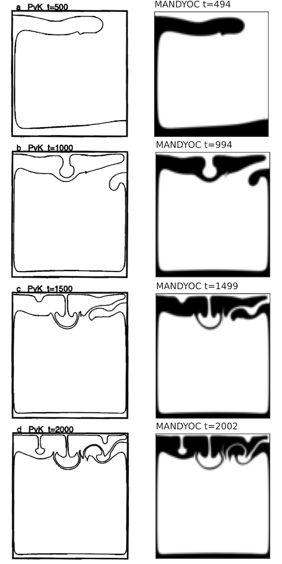
Fig. 6.1 Evolution of the isoviscous Rayleigh-Taylor instability for \(\eta_0/\eta_r=1.00\). The best result presented by van Keken et al. (1997) [20] are on the left and the Mandyoc results are on the right.

Note

Because of the different methods used by van Keken et al. (1997) [20] and Mandyoc, the Mandyoc results for the evolution of the isoviscous Rayleigh-Taylor instability presents its data colored instead of contoured.

Fig. 6.2 below compares the change of the \(v_{rms}\) with time, showing the results from van Keken et al. (1997) [20] in gray and Mandyoc in black.

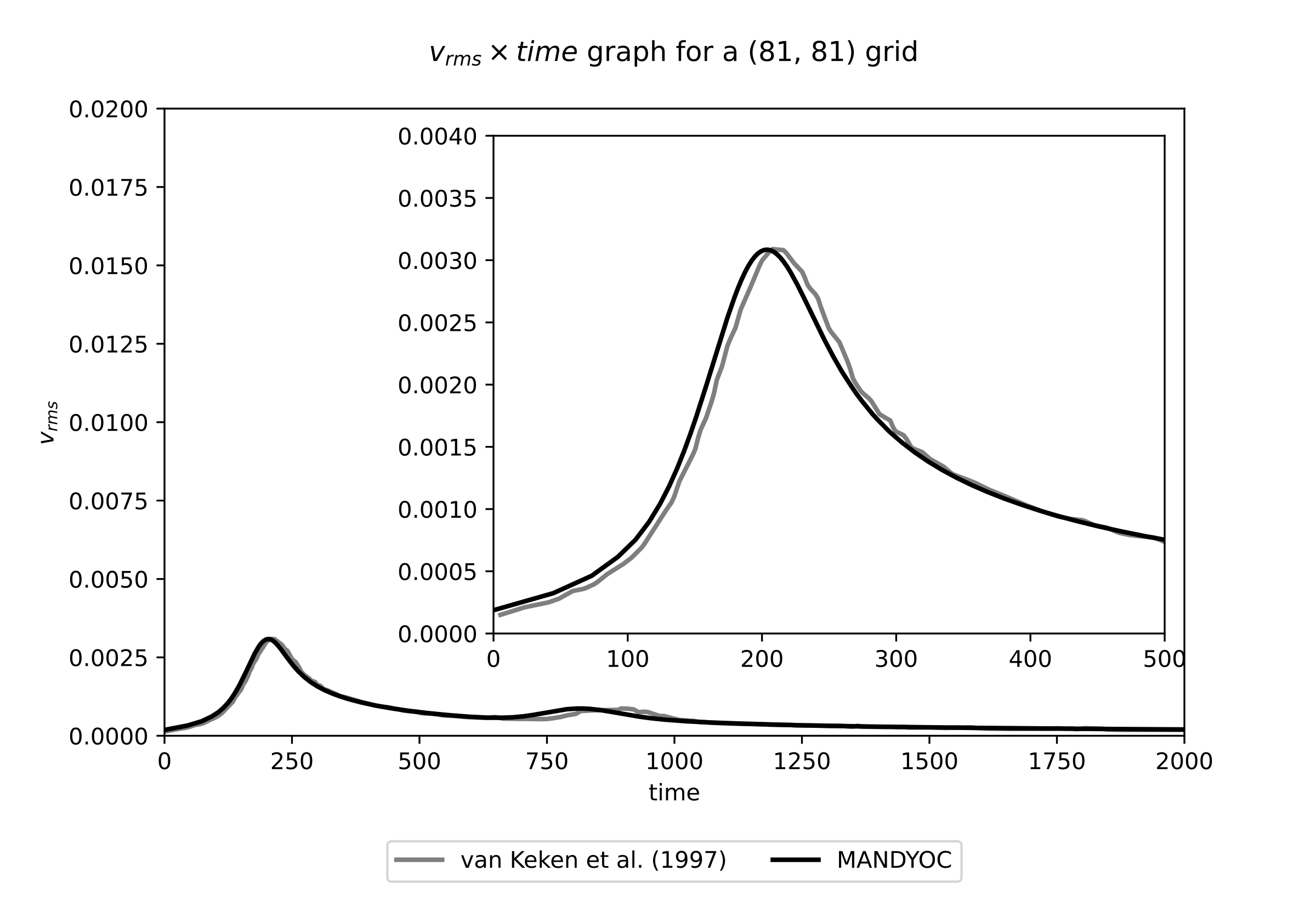
Fig. 6.2 Evolution of the \(v_{rms}\) for \(\eta_0/\eta_r=1.00\). The van Keken et al. (1997) [20] result is shown in black and the Mandyoc code result is shown in gray.

6.1.2. Results for case 1b

For the case 1b where \(\eta_0/\eta_r=0.10\), Fig. 6.3 compares the evolution of the isoviscous Rayleigh-Taylor instability between van Keken et al. (1997) [20] and Mandyoc. The time steps shown for the Mandyoc code are the closest the simulation could provide, considering the chosen simulation parameters.

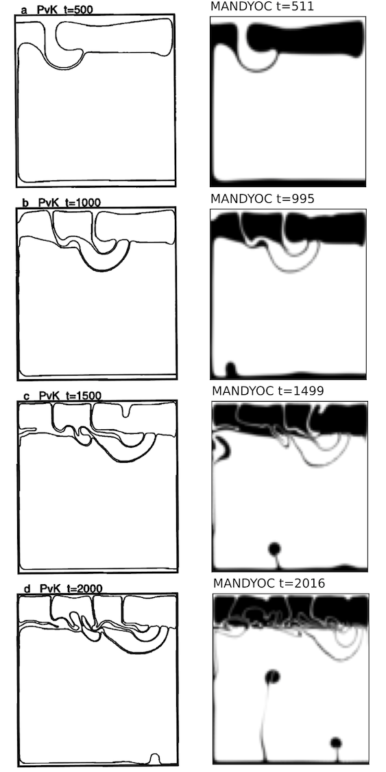
Fig. 6.3 Evolution of the isoviscous Rayleigh-Taylor instability for \(\eta_0/\eta_r=0.10\). The best result presented by van Keken et al. (1997) [20] are on the left and the Mandyoc results are on the right.

Fig. 6.4 below compares the change of the \(v_{rms}\) with time, showing the results from van Keken et al. (1997) [20] in gray and Mandyoc in black.

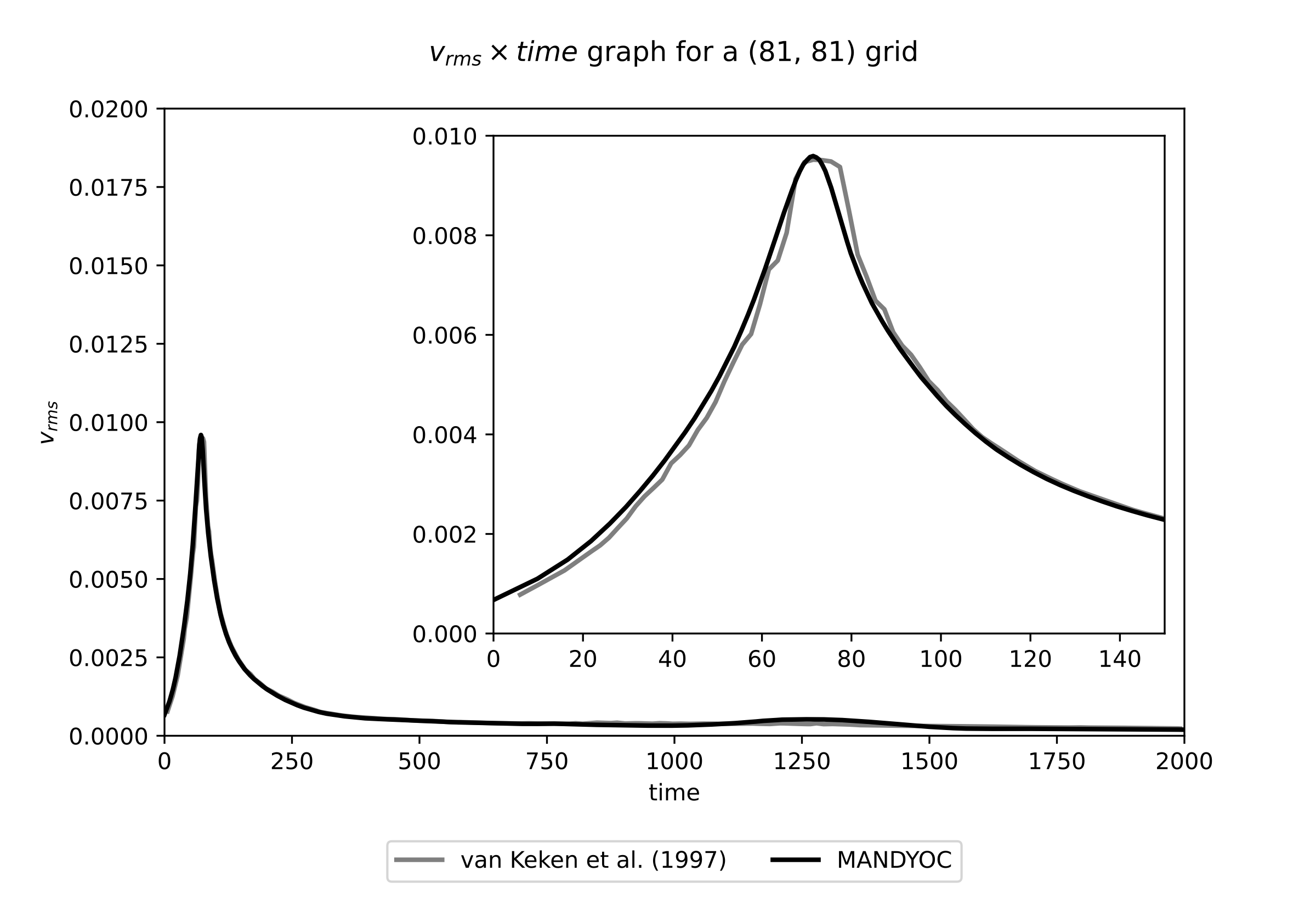
Fig. 6.4 Evolution of the \(v_{rms}\) for \(\eta_0/\eta_r=0.10\). The van Keken et al. (1997) [20] result is shown in black and the Mandyoc code result is shown in gray.

6.1.3. Results for case 1c

For the case 1c where \(\eta_0/\eta_r=0.01\), Fig. 6.5 compares the evolution of the isoviscous Rayleigh-Taylor instability between van Keken et al. (1997) [20] and Mandyoc. The time steps shown for the Mandyoc code are the closest the simulation could provide, considering the chosen simulation parameters.

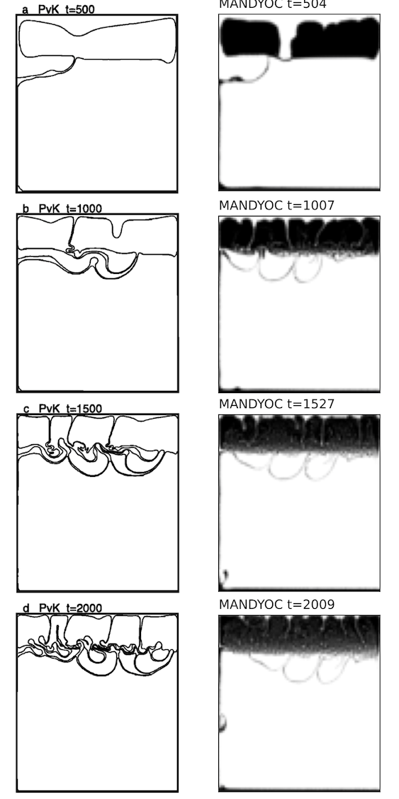
Fig. 6.5 Evolution of the isoviscous Rayleigh-Taylor instability for \(\eta_0/\eta_r=0.01\). The best result presented by van Keken et al. (1997) [20] are on the left and the Mandyoc results are on the right.

Fig. 6.6 below compares the change of the \(v_{rms}\) with time, showing the results from van Keken et al. (1997) [20] in gray and Mandyoc in black.

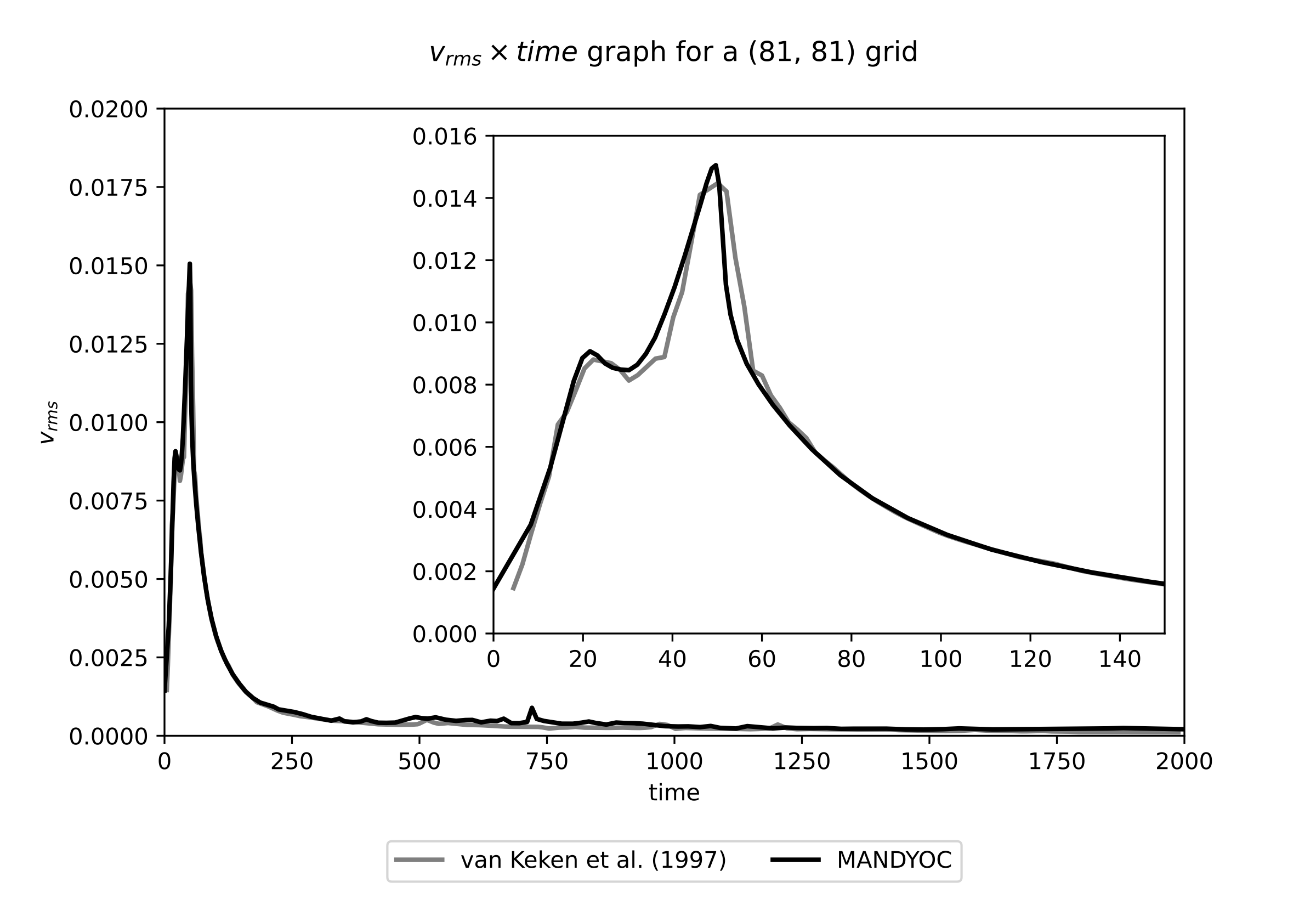
Fig. 6.6 Evolution of the \(v_{rms}\) for \(\eta_0/\eta_r=0.01\). The van Keken et al. (1997) [20] result is shown in black and the Mandyoc code result is shown in gray.

6.1.4. Basic scaling

Below, Fig. 6.7 shows the results of a basic scaling test for Mandyoc (v.0.1.4) running on Intel(R) Core(TM) i7-10700 CPU @ 2.90GHz.

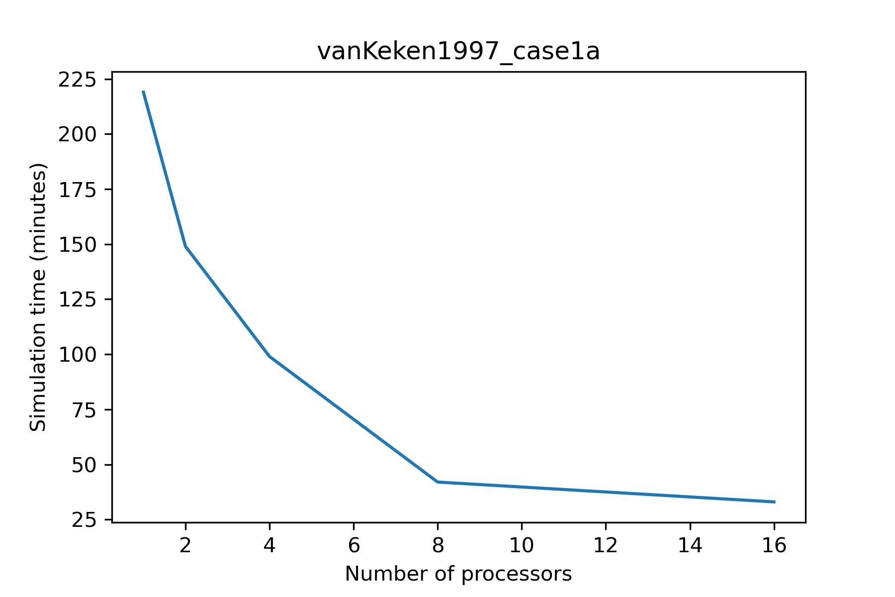
Fig. 6.7 Results of scaling test for vanKeken1997_case1a.

6.2. Crameri et al. (2012) [21]

Note

Mandyoc version used for this benchmark: v0.1.4.

The Case 2 experiment presented by Crameri et al. (2012) [21] evaluates the sticky air method to obtain a numerical surface topography in geodynamic modelling.

The experiment analyses the change in topography due to the rising of a mantle plume. The model setup (Fig. 6.8) consists of a \(2800 \, \mathrm{km}\) by \(850 \, \mathrm{km}\) box with a \(150 \, \mathrm{km}\) sticky air layer on the top of the model. The mantle thickness is \(600 \, \mathrm{km}\) with a \(100 \, \mathrm{km}\) thick lithosphere. The lithosphere density is \(3300 \, \mathrm{kg/m}^3\) with viscosity \(10^{23} \, \mathrm{Pa\,s}\), the mantle density is \(3300 \, \mathrm{kg/m}^3\) with viscosity \(10^{21} \, \mathrm{Pa\,s}\) and the mantle plume density is \(3200 \, \mathrm{kg/m}^3\) with viscosity \(10^{20} \, \mathrm{Pa\,s}\). Initially, the center of the plume is horizontally centered and \(300 \, \mathrm{km}\) above the base of the model. At the top, the sticky air layer has density \(0 \, \mathrm{kg/m}^3\) with viscosity \(10^{19} \, \mathrm{Pa\,s}\). A free slip boundary condition is applied to the upper boundary of the sticky air layer and the vertical sides of the model and the base is kept fixed. There is no temperature difference, and the geodynamic evolution is guided solely by compositional density differences.

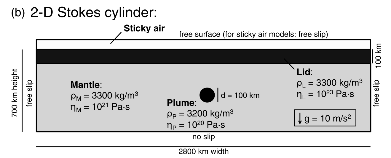
Fig. 6.8 Case 2 model setup to evaluate the sticky air method. Extracted from Crameri et al. (2012) [21].

From the results of this experiment reproduced in MANDYOC we obtain the maximum topography with time, similar to Fig. 6a of Crameri et al. (2012) [21], presented in Fig. 6.9. The models used for comparison are: UNDERWORLD [22], STAGYY [23] and I2VIS [24]. The data used for comparison was extract from Crameri et al. (2012), which used UNDERWORLD v1.5.0. No version information for STAGYY and I2VIS codes was reported.

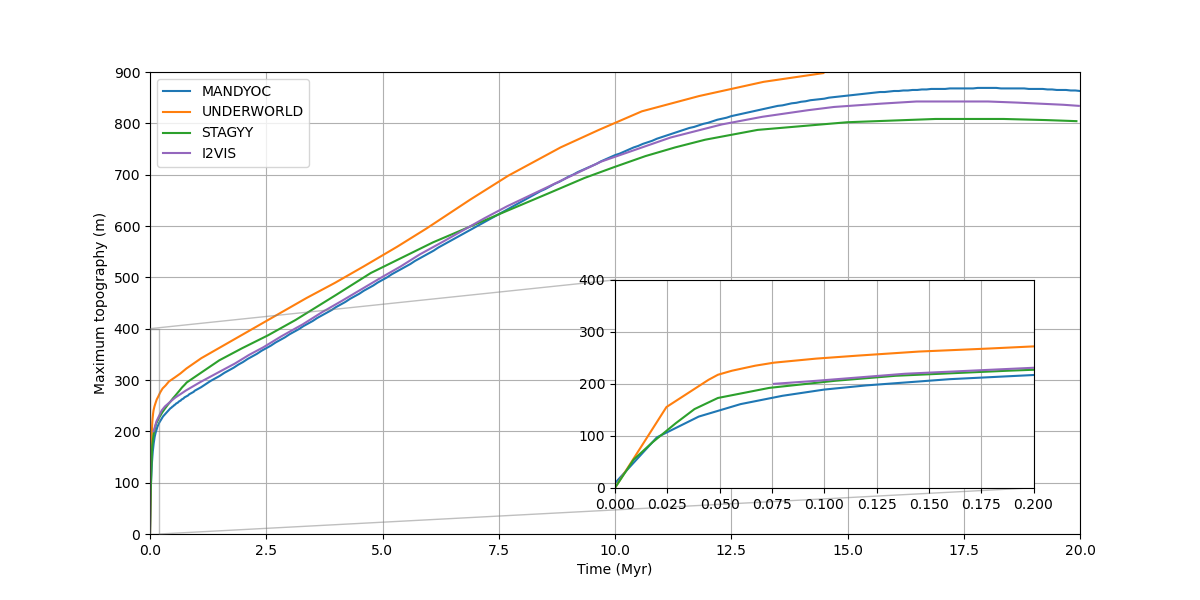
Fig. 6.9 Comparison of the maximum topography with time for the Case 2 (Fig. 6.8) model setup from Crameri et al. (2012) [21].

6.2.1. Basic scaling

Below, Fig. 6.10 shows the results of a basic scaling test for Mandyoc (v.0.1.4) running on Intel(R) Core(TM) i7-10700 CPU @ 2.90GHz.

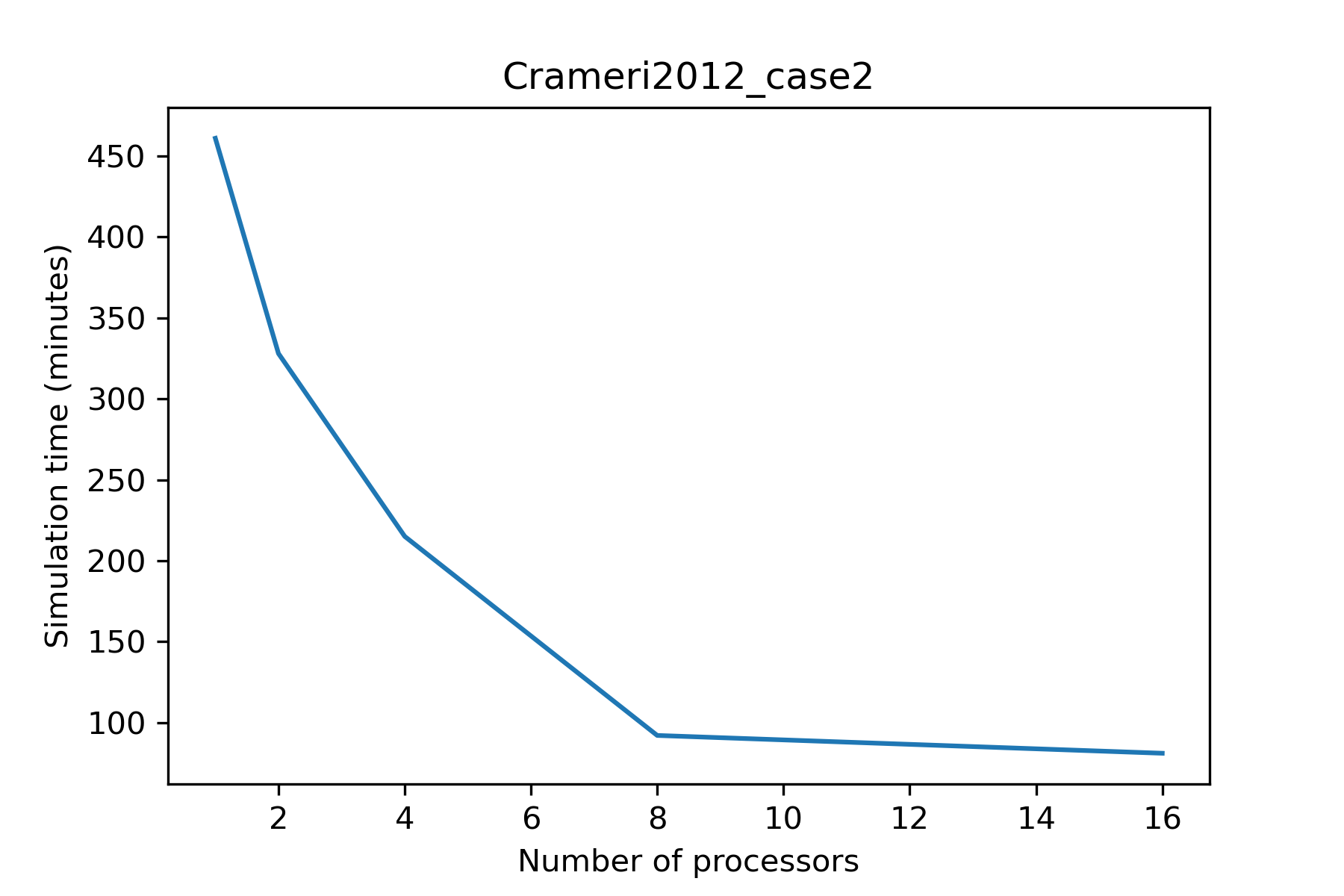
Fig. 6.10 Results of scaling test for Crameri2012_case2.

6.3. The indenter benchmark

In this problem, a rigid punch vertically indents a rigid plastic half space. This problem presents an analytical solution

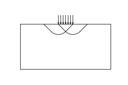
Fig. 6.11 Applied boundary conditions and the expected slip-lines.

The numerical simulation is performed only for one time step in a material with pure plastic von Mises rheology (Thieulot et al., 2008) [25]. The yield function \(F\) is

\(F = 2 \eta \dot\varepsilon_{II} - 1\)

where \(\eta\) is the viscosity and \(\dot\varepsilon_{II}\) is the square root of the second invariant of the deviatoric strain rate tensor.

If \(F>0\), the stress is outside the yield surface, and the effective viscosity \(\eta_{eff}\) is

\(\eta_{eff} = \frac{1}{2\dot\varepsilon_{II}}\).

The horizontal and vertical dimensions of the domain are set to \(L_x = 1\) and \(L_y = 0.5\). The left and right boundaries are set to free slip and the bottom to no slip. At the top boundary, the velocity is prescribed as (0,-1) in the center of the domain, in the interval \(L_x/2-\delta_x\) and \(L_x/2+\delta_x\) with \(\delta_x = 0.08\). Outside this interval, the velocity on the top boundary was set free. The minimum and maximum effective viscosity were set as \(10^{-2}\) and \(10^4\), respectively.

The results presented in the following figures were obtained from a numerical simulation performed with a mesh with 400x200 elements.

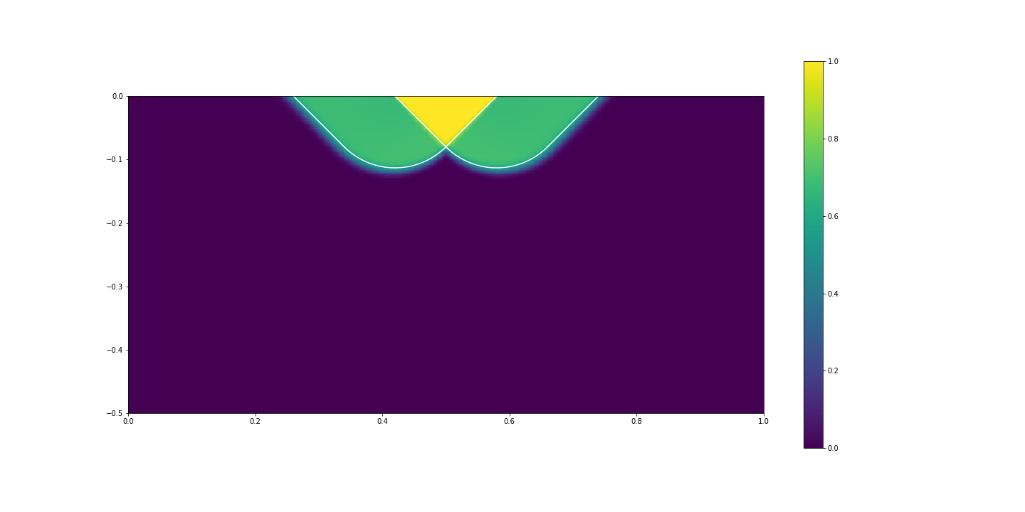
Fig. 6.12 Absolute value for the velocity field. The white curves are the slip-lines from the analytical solution.

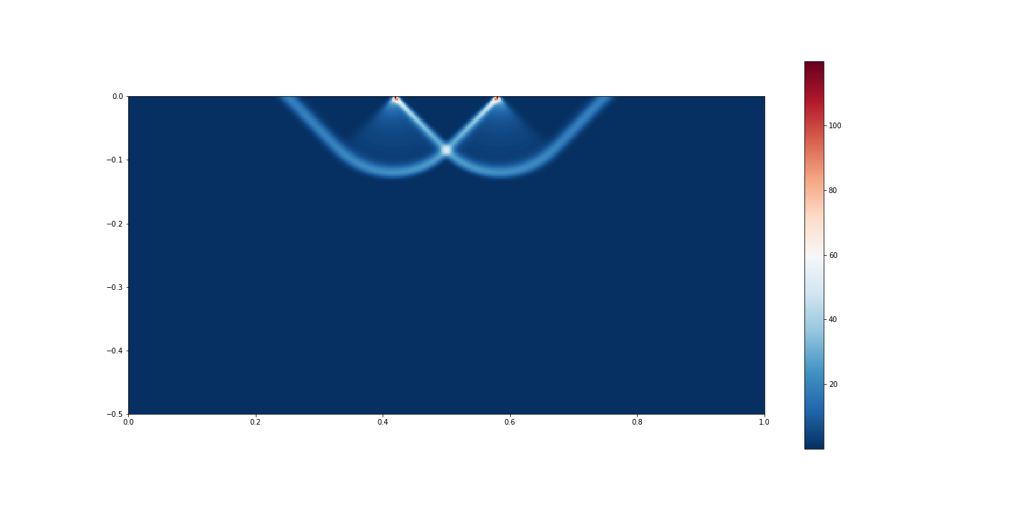
Fig. 6.13 Strain rate field.

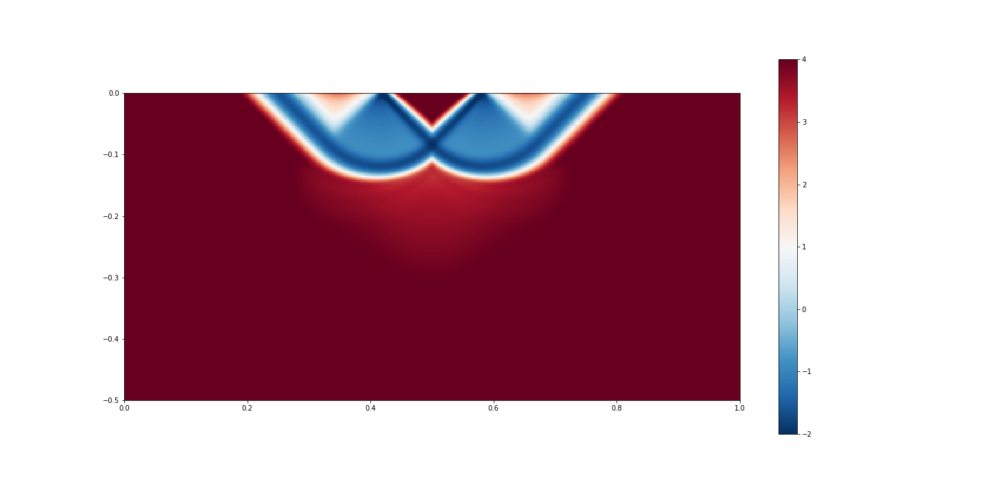
Fig. 6.14 Logarithm of the Viscosity field.

The shear bands obtained with the numerical simulation follows the slip lines at \(\pi/4\) angle, as predicted by the analytical solution (indicated by the white lines in the figure for the velocity field), separating the three rigid bodies.

6.4. The slab detachment benchmark

Here we test the slab detachment model proposed by Schmalholz (2011) [26]. It assumes a nonlinear viscous rheology for the lithosphere, with the viscosity \(\eta\) function of the square root of the second invariant of the deviatoric strain rate tensor \(\dot\varepsilon_{II}\):

\(\eta = \eta_0 \dot\varepsilon_{II}^{(1/n-1)}\)

where \(\eta_0 = 4.75 \times 10^{11}\) Pa s^1/n and \(n=4\).

Under the lithosphere, the mantle presents constant viscosity (\(\eta_{mantle} = 10^{21}\) Pa s).

The domain width is 1000 km and the domain height is 660 km. The lithosphere on the top of the domain is 80 km thick. In the center of the domain, a vertical slab 80-km thick and 250-km long is attached to the base of the lithosphere.

The density of the rocks are not dependent on temperature, assumed constant during all the numerical simulation: 3300 kg/m³ for the lithosphere and 3150 kg/m³ for the sublithospheric mantle. The gravity acceleration is 9.81 m/s².

During the numerical simulation, the slab is stretched by its own weight, resulting in the necking in the upper portion of the slab.

Snapshots in different moments are shown below:

Fig. 6.15 Viscosity structure - \(\log_{10} (\eta)\), with \(\eta\) in Pa s.

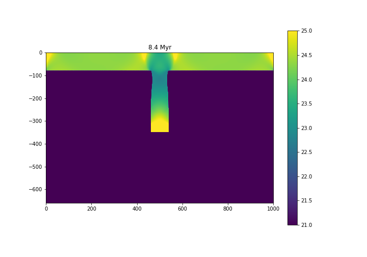
Fig. 6.16 Viscosity structure - \(\log_{10} (\eta)\), with \(\eta\) in Pa s.

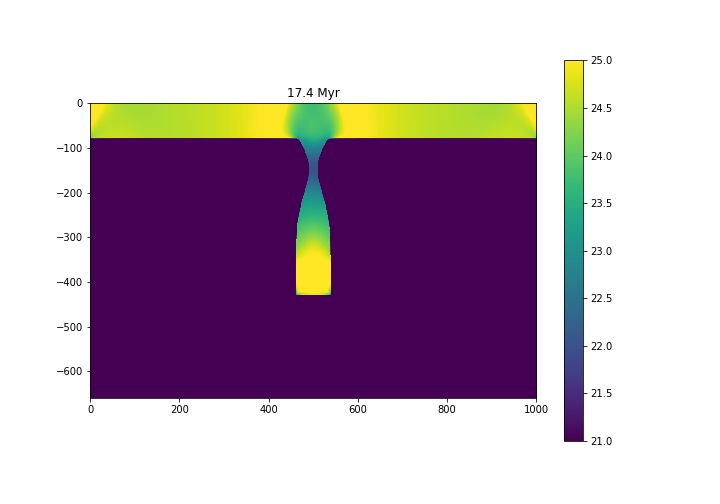
Fig. 6.17 Viscosity structure - \(\log_{10} (\eta)\), with \(\eta\) in Pa s.

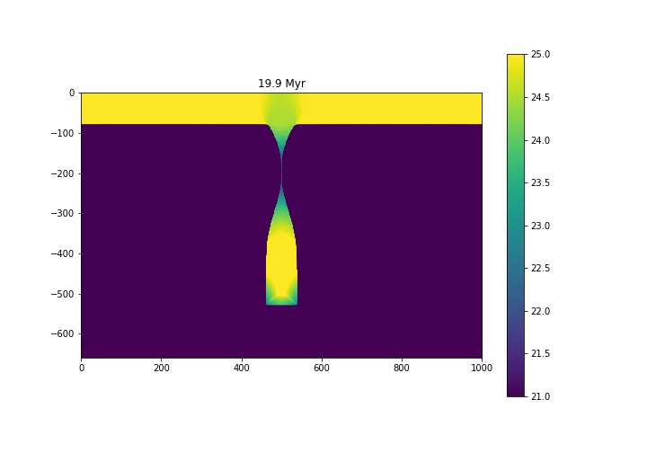
Fig. 6.18 Viscosity structure - \(\log_{10} (\eta)\), with \(\eta\) in Pa s.

To study the evolution of the necking of the slab and compare with previous works, we normalized the necking width to the initial thickness of the slab (80 km). Additionally, the time was divided by the characteristic time \(t_c = 7.1158\times10^{14}\) s (Glerum et al., 2008 [27]).

The following figure shows the necking width through time, compared with the results from Schmalholz (2011) [26] and Glerum et al. (2008) [27]:

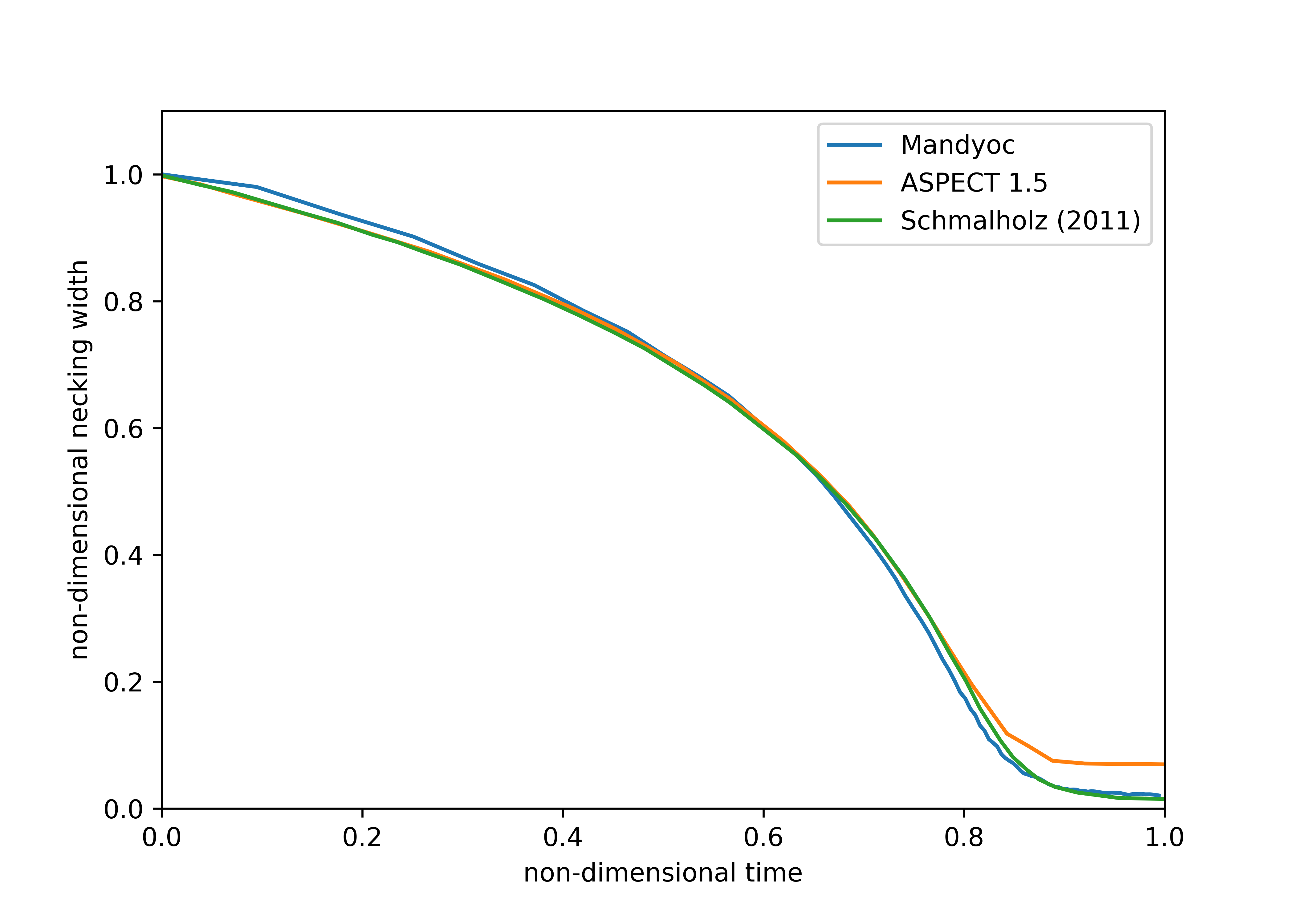
Fig. 6.19 Necking width through time