5. Input files
Mandyoc accepts ASCII files to use as initial conditions for the simulation, such as an initial temperature file input_temperature_0.txt, a file containing the initial interfaces geometry interfaces.txt and a file containing the initial velocity field at the faces of the model input_velocity_0.txt. The next subsections will help you creating each one of these files.
5.1. ASCII temperature file
For a 2-D grid, the initial temperature configuration can be provided as an ASCII file called input_temperature_0.txt. Considering \(x\) to be the longitudinal direction and \(y\) the vertical direction, the next subsections will guide you through the understanding of the initial temperature file structure.
5.1.1. 2-D temperature grid
Consider a 2-D grid where the number of nodes in the \(x\) and \(y\) directions are \(nx\geq 2\) and \(ny\geq 2\), respectively, with \((nx-1)\) elements in the \(x\) direction and \((ny-1)\) elements in the \(y\) direction. Each node in the grid can be identified with a coordinates pair \((x_n, y_m)\), where \(n\) and \(m\) are natural numbers, and \(x_n\) and \(y_m\) are the \(x\) and \(y\) positions (in meters) of any grid node. Fig. 5.1 shows a scheme for a 2-D grid, where the red dots represent the grid nodes and every node is labeled with a \((x_n, y_m)\) pair. The dotted lines represent any number of intermediate nodes.
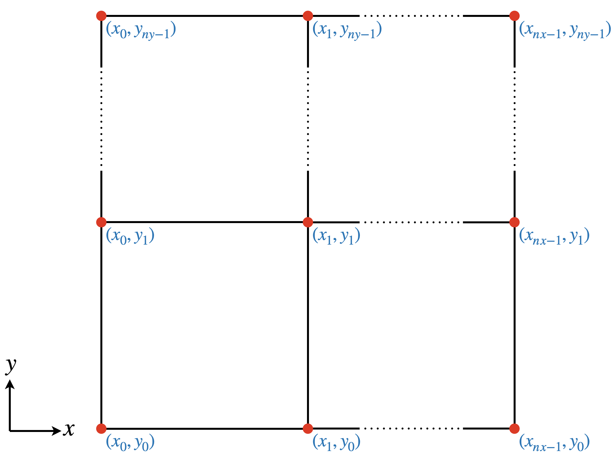
Fig. 5.1 2-D grid scheme. The red dots represent the grid nodes where the values for the temperature must be defined, the dotted lines represent any number of grid nodes, for simplification, and the labels indicate the \(x\) and \(y\) position of each node.
Note
Because of the way Mandyoc deals with the coordinates in 2-D, the node at \((x_0,y_0)\) is always at the origin \((0,0)\).
The example below shows how the input_temperature_0.txt file must be written for the 2-D grid in Fig. 5.1: after writing four lines of comments, the file must include the temperature \(T(x_n, y_m)\) at each node starting at the bottom left of the model and going up in the \(y\) direction. Intuitively, the temperature is given in horizontal layers for every \(x_n\).
 1# Header line 0
 2# Header line 1
 3# Header line 2
 4# Header line 3
 5T(x_0, y_0)
 6T(x_1, y_0)
 7T(x_2, y_0)
 8T(x_3, y_0)
 9[...]
10T(x_{nx-1}, y_0)
11T(x_0, y_1)
12T(x_1, y_1)
13T(x_2, y_1)
14T(x_3, y_1)
15[...]
16T(x_{nx-1}, y_1)
17T(x_0, y_2)
18T(x_1, y_2)
19T(x_2, y_2)
20T(x_3, y_2)
21[...]
22T(x_{nx-1}, y_2)
23T(x_0, y_3)
24T(x_1, y_3)
25T(x_2, y_3)
26T(x_3, y_3)
27[...]
28T(x_{nx-1}, y_3)
29[...]
30T(x_0, y_{ny-1})
31T(x_1, y_{ny-1})
32T(x_2, y_{ny-1})
33T(x_3, y_{ny-1})
34[...]
35T(x_{nx-1}, y_{ny-1})
Tip
It is always helpful to use the four comment lines to write down any useful information for later. Because these lines are simply skipped, there is no rule to write them, the ‘#’ symbol is used only by convention.
5.2. ASCII interfaces file
The interfaces.txt file, for a 2-D grid, starts with seven lines of variables that are used by the rheology models. The variables that are in the interfaces are those that might be used in Eq. 2.32 or Eq. 2.31: \(C\), \(\rho_r\), \(H\), \(A\), \(n\), \(Q\), and \(V\). Each one of these variables possesses a number of values (columns) that are assigned to each lithological unit in the model. Every interface is a boundary between two lithological units, therefore the number of columns is 1 plus the number of interfaces set in the param.txt file (see the parameter file section), such that if there are \(i\) interfaces, \(i+1\) values for each variable must be provided in the interfaces.txt file. More will be discussed about the order of these values shortly.
5.2.1. 2-D Initial interfaces
Below, the example corresponds to a 2-D grid with two interfaces and, therefore, three lithological units. The first column contains the vertical positions in meters of every grid node \(y_m\) that corresponds to the deepest interface boundary, starting at \(x=x_0\) on line 8, and ending at \(x=x_{nx-1}\) on line \(nx+7\). The second column contains the vertical position of every \(y_m\) that corresponds to the second interface boundary. When defining the interfaces, it is rather common for them to “touch”. Because of that, all the interfaces must be provided in a “tetris” manner, where interfaces that are collinear in parts fit the interface below.
Note
Because the interfaces are defined linearly between the nodes, it is important to define them properly, so every point inside the grid can be attributed to a lithological unit.
 1C    1.0    1.0    1.0
 2rho  3000.0 3000.0 3000.0
 3H    0.0    0.0    0.0
 4A    0.0    0.0    0.0
 5n    0.0    0.0    0.0
 6Q    0.0    0.0    0.0
 7V    0.0    0.0    0.0
 8y_1(x_0)    y_2(x_0)
 9y_1(x_1)    y_2(x_1)
10y_1(x_2)    y_2(x_2)
11y_1(x_3)    y_2(x_3)
12y_1(x_4)    y_2(x_4)
13y_1(x_5)    y_2(x_5)
14y_1(x_6)    y_2(x_6)
The values of the variables in the first seven lines are the values of the lithological units bound by the interfaces. For the 2-D grid with two interfaces, the first values of each variable refers to the lithological unit below the first interface, the second value of each variable refers to the lithological unit between the first and second interfaces, and the third value of each variable refers to the lithological unit above the second interface. If more interfaces are added, there will be more units bounded by an upper and a lower interface.
To consider different values of internal cohesion \(c_0\) and internal angle of friction \(\varphi\) for each layer, the interface file can be written as the file below, where weakening_seed, cohesion_min, cohesion_max, friction_angle_min, and friction_angle_max are given.
 1C    				1.0    1.0    1.0
 2rho  				3000.0 3000.0 3000.0
 3H    				0.0    0.0    0.0
 4A    				0.0    0.0    0.0
 5n    				0.0    0.0    0.0
 6Q    				0.0    0.0    0.0
 7V    				0.0    0.0    0.0
 8weakeing_seed		1.0    -1.0   0.5
 9cohesion_min		5.0e6  5.0e6  5.0e6
10cohesion_max		30.0e7 5.0e6  1.0e7
11friction_angle_min	0.0    0.2    10.0
12friction_angle_max	0.0    20.0   10.0
13y_1(x_0)    y_2(x_0)
14y_1(x_1)    y_2(x_1)
15y_1(x_2)    y_2(x_2)
16y_1(x_3)    y_2(x_3)
17y_1(x_4)    y_2(x_4)
18y_1(x_5)    y_2(x_5)
19y_1(x_6)    y_2(x_6)
The weakening_seed value for each layer represents its initial accumulated strain value (seed), and when it is negative, a random seed will be used instead. When cohesion_min and cohesion_max are different, that corresponding layer will be linearly softened between those values. Notice that a constant cohesion can be set if the values are simply equal. The same logic aplies to friction_angle_min and friction_angle_max.
The default interval of accumualted strain where strain softening occurs is 0.05 and 1.05, cf. [19]. To use different values, the user must provide them in the param.txt withe the keywords weakeing_min and weakening_max.
5.3. ASCII velocities files
An initial velocity file allows an initial velocity field to be established so the simulated fluid presents an initial momentum. Respecting the conservation of mass equation when designing the initial velocity field is fundamental so the simulation can run properly.
Additionally, the velocity boundary conditions defined in the param.txt (see the parameter file section) will be used to define the normal and tangential velocities on the faces of the model during the simulation.
5.3.1. 2-D initial velocity
When velocity_from_ascii = True is set in the param.txt file, an initial velocity field must be provided in an ASCII file called input_velocity_0.txt.
For a 2-D grid, the input_velocity_0.txt file possesses four lines of headers followed by the velocity data for each node of the model. The velocity must be defined for both \(x\) and \(y\) directions. Taking the example in the file below, the input_velocity_0.txt file must be written in such a way that the values for the velocity in the \(x\) direction \(v_x\) and the velocity in the \(y\) direction \(v_y\) for the node \((x_0,y_0)\) corresponds to lines 5 and 6, respectively, the velocity values for the \((x_1,y_0)\) corresponds to lines 7 and 8, and so on until \((x_{nx-1},y_0)\). Once all the nodes in the \(y_0\) are written, the values for all \(x_n\) are inserted for \(y_1\), and so on until \(y_{ny-1}\).
 1# Header line 0
 2# Header line 1
 3# Header line 2
 4# Header line 3
 5v_x(x_0,y_0)
 6v_y(x_0,y_0)
 7v_x(x_1,y_0)
 8v_y(x_1,y_0)
 9v_x(x_2,y_0)
10v_y(x_2,y_0)
11[...]
12v_x(x_{nx-1},y_0)
13v_y(x_{nx-1},y_0)
14v_x(x_0,y_1)
15v_y(x_0,y_1)
16v_x(x_1,y_1)
17v_y(x_1,y_1)
18v_x(x_2,y_1)
19v_y(x_2,y_1)
20[...]
21v_x(x_{nx-1},y_1)
22v_y(x_{nx-1},y_1)
23[...]
24v_x(x_0,y_{ny-1})
25v_y(x_0,y_{ny-1})
26[...]
27v_x(x_{nx-1},y_{ny-1})
28v_y(x_{nx-1},y_{ny-1})
5.3.2. 2-D multiple initial velocities
The user can provide multiple velocity fields to be set in different instants of the simulation. By setting multi_velocity = True in the param.txt file, an ASCII file called multi_veloc.txt must be provided following the structure shown in the example file below. The first line of the file contains the amount of instants where a different velocity field will be used and the other lines contain the time, in millions of years, that each velocity field will be adopted. In the example below, a different velocity field will be used at three instants, the files must follow the structure presented in the last section and should be named in sequence: input_velocity_1.txt, input_velocity_2.txt and input_velocity_3.txt. The names of the files are labeled after the three different instants set in the first line of the multi_veloc.txt file.
13
210.0
325.0
450.0
Note
The input_velocity_0.txt is used for the beginning of the simulation. The multiple initial velocities that can be set during the simulation start at input_velocity_1.txt and end at input_velocity_X.txt, where \(X\) is the number of different instants that the velocity field will be changed.
5.3.3. 2-D re-scalable boundary condition
When variable_bcv = True is set in the param.txt``file, an ASCII file called ``scale_bcv.txt is used to define a sequence of re-scaling steps for the velocity boundary conditions. The example file below is an example of how such file can be written. In the example file, the first line corresponds to the number of instants during the simulation that the velocity field will be re-scaled. The first column contains the time, in millions of years, that the velocity field will be changed and the second column contains the scale value. For the example below, in the instant \(10.0\) Myr the velocity field will be multiplied by \(0.5\), effectively halving it; at \(25.0\) Myr the current velocity field will have its direction changed, hence multiplied by \(-1.0\); and finally at \(50\) My the velocity field will have its direction changed again and doubled by multiplying it by \(-2.0\).
13
210.0     0.5
325.0    -1.0
450.0    -2.0